

Many of you have probably heard the phrase ‘data is the new oil’, and that is because everything in our world produces valuable information. It is up to us to be able to extract value from all the noisy and messy data that is being produced every moment.
But working with data is not easy: as we have seen before, real data is always noisy, messy and often incomplete, and even the extraction process sometimes suffers from some flaws.
It is therefore very important to make the data usable through a process known as data wrangling (i.e. the process of cleaning, structuring and enriching the raw data into the desired format) to improve decision-making. The crucial aspect to understand is that bad data leads to bad decisions, so it is important to make this process stable, repeatable and idempotent to ensure that our transformations improve the quality of the data and not degrade it.
Let’s look at one aspect of the data wrangling process: how to deal with data sources that cannot guarantee the quality of what they provide.
The Context
In a recent project in which we were involved, we faced a scenario in which the data sources were highly unreliable.
According to initial definitions, the expected data from a range of sensors should have been:
- about ten different types of data
- each type at a fixed rate (every 10 minutes)
- data will arrive in a landing bucket
- data will be in CSV format, with a predefined schema and a fixed number of rows.
From this data, we would perform validation, cleaning and aggregation in order to calculate certain KPIs. These KPIs were the starting point for a subsequent forecast based on Machine Learning.
In addition, it was necessary to produce reports and forecasts updated every 10 minutes with the latest information received.
As in many real projects in the data world, the source data had several problems, such as missing data in the CSV (sometimes some values were missing in some cells, whole rows were missing, or duplicate rows were missing), or data arriving late (even not arriving at all).
The Solution
In such scenarios, it is crucial to keep track of the transformations that the data pipeline will apply and to be able to answer questions such as these:
- what are the source values of a given result?
- does the value of a result come from actual data or from imputed data?
- all sources arrived in time?
- how reliable is a given result?
In order to answer this type of question, we must first isolate the different types of data in at least three areas:
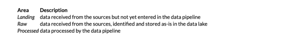
In particular, the Landing Area is a place where external systems (i.e. data sources) write, while the data pipeline can only read or delete after a safe retention time.
In the Raw Area, on the other hand, we will copy CSVs from the Landing Area keeping the data as is, but enriching the metadata (e.g. labelling the file or putting it into a better organised folder structure). This will be our Data Lake from which we will always be able to retrieve the original data, either in the event of errors during processing or when developing a new feature.
Finally, in the Processed Area we store the validated and cleaned data. This area will be the starting point for the Visualisation component and the Machine Learning component.
Having defined the three previous areas for storing data, we must introduce another concept that allows us to track information through the pipeline: the Run Control Value.
The execution control value is a metadata, often a serial value or timestamp, or whatever, and gives us the ability to correlate the data in the different areas with the executions in the pipeline.
This concept is simple enough to implement, but not so obvious to understand. On the other hand, it is easy to be misled; some might think it is superfluous and can be removed in favour of information already present in the data, such as a timestamp, but that would be wrong.
Let us now see, with some examples, the advantages of using the data separation described above, together with the Run Control Value.
Example 1: Tracking Data Imputation
Let us first consider a scenario in which the output is strange and looks apparently wrong. The RCV column represents the Run Control Value and is added by the pipeline.
Here we can see that, if we only look at the processed data, for the input at 11:00 the entry with ID=2 is missing, and the counter with ID=1 has a strange zero as a value (suppose our domain expert said that the zeros in the counter column are anomalous).
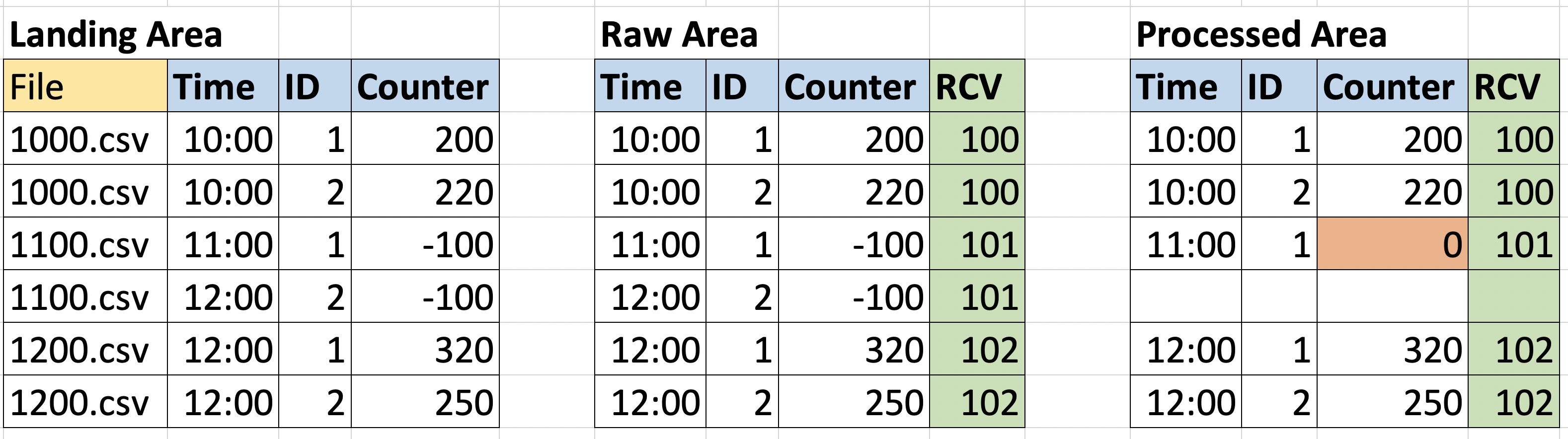
In this case, we can trace the steps in the pipeline, using the Run Control Value, and see which values actually contributed to the output, whether all inputs were available at the time the calculation was performed, or whether some files were missing in the Raw Area and thus were completed with the imputed values.
In the image above, you can see that in the Raw area, the inputs with RCV=101 were both negative, and the entity with ID=2 is related to time=12:00. If you then check the original file in the Landing Area, you can see that this file was named 1100.csv (in the image represented as a pair of table rows for simplicity), so the entry for time 12:00 was an error; the entry was therefore removed in the Processed Area, while the other was reset by an imputation rule.
The solution of keeping the Landing Area separate from the Raw Area also allows us to handle the case of late arriving data.
Given the scenario described at the beginning of the article, we receive the data in batch with a scheduler driving the ingestion. So what happens if, at the time of the scheduled ingestion, one of the inputs was missing and was met with imputed values, but, at debug time, we can see that it is available?
In this case, it will be available in the Landing Area but will be missing in the Raw area; therefore, without even opening the file to check the values, we can quickly realise that for that specific run, those values have been imputed.
Example 2: Error from Sources with Resubmission of Input Data
In the first example, we discussed retrospectively analysing processing or debugging. Let us now consider another case: a source with a problem sent incorrect data in a certain execution; after the problem has been solved, we want to re-analyses the data for the same execution to update our output, and re-execute it in the same context.
The following image shows the status of the data warehouse when the input at 11.00 a.m. has a couple of problems: the entry with ID=2 is missing and the entryID=1 has a negative value and we have a validation rule to convert negative values to zero. So the Processed Area table contains the validated data.
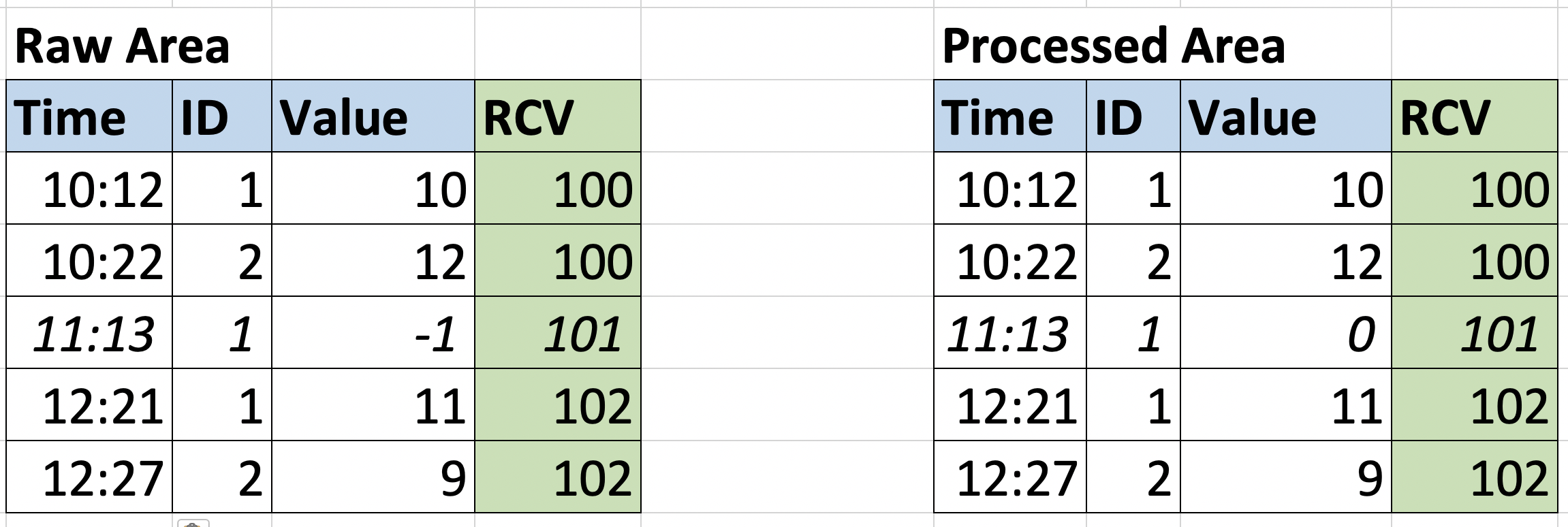
In the correct version of the file, there is a valid entry for each entity. The pipeline will use RCV=101 as a reference to clean up the table from the previous execution and ingest the new file.
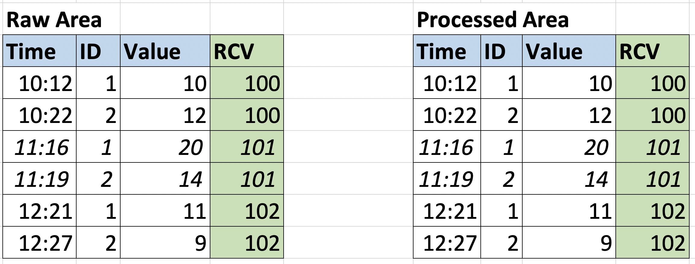
In this case, the Run Control Value allows us to identify precisely which portion of data was ingested with the previous execution, so that we can safely remove it and re-execute with the correct one.
These are just two simple scenarios that can be addressed with this technique, but many other data pipeline problems can benefit from this approach.
Furthermore, this mechanism allows us to have the idempotence of the stages of the pipeline, i.e. the possibility of tracing the data passing through the different stages, and reapplying the transformations on the same input and obtaining the same result.
Conclusions
In this article, we dived a little into the world of data engineering, discovering in particular how to handle data from unreliable sources, most often in real projects.
We have seen why phase separation is important in designing a data pipeline and also what properties each ‘area’ will have; this helps us better understand what is going on and identify potential problems.
Another aspect we have highlighted is how this technique facilitates the handling of data that arrives late or the re-engineering of correct data, in case a problem can be solved at source.
Autore: Luca Tronchin, Software Engineer @Bitrock